Reading on Quicksort
Quicksort: An Example of Divide-and-Conquer Algorithms and the
Use of Loop Invariants in Code Development
Initial Notes:
-
The quicksort was originally devised by C. A. R. Hoare. For more details,
see the Computing Journal, Volume 5 (1962), pages 10-15.
-
The basic approach involves applying an initial step that partitions an
array into two pieces. The algorithm then is applied recursively to each
of the two pieces. This approach of dividing processing into pieces and
applying recursion to the two pieces turns out to be extremely general and
powerful. Such an approach is called a divide and conquer
algorithm.
-
Even given the central approach for the overall algorithm,
several variations have been proposed for a central procedure,
called partition. In practice, the major differences in
these alternatives relate to underlying conditions that are
maintained for a main loop. These conditions are called loop
invariants.
Credits:
-
Much of the following discussion is based on the presentation in
Henry M. Walker, Pascal: Problem Solving and Structured Program
Design, Little, Brown, and Company, 1987, pages 500-506, and is
used with permission of the copyright holder.
-
The alternative loop invariant discussed below is based on
Thomas H. Cormen, Charles E. Leiserson, Ronald L. Rivset, and Clifford
Stein, Introduction to Algorithms, Third Edition The MIT Press, 2009,
pages170-185.
-
Variations of a third loop invariant are discussed in several
YouTube videos.
Overview
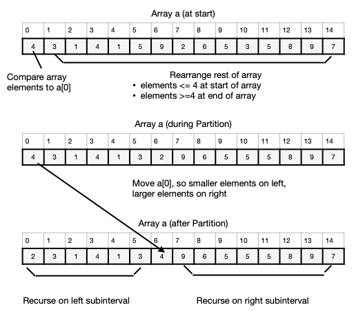
The quicksort is a recursive approach to sorting, and we begin by outlining
the principal recursive step. In this step, we make a guess at the value
that should end up in the middle of the array. In particular, given the
array a[0], ..., a[N-1] of data, arranged at random, then we might guess
that the first data item a[0] often should end up in about the middle of
the array when the array is finally ordered. (a[0] is easy to locate, and
it is as good a guess at the median value as another.) This suggests the
following steps:
-
Rearrange the data in the a array, so that A[0] is moved to its proper
position. In other words, move a[0] to a[mid], for an appropriate
index mid, and rearrange the other
elements so that:
a[0], a[1], ..., a[mid-1] <- a[mid]
and
a[mid] <= a[mid+1], ..., a[N-1].
-
Repeat this process on the smaller lists
a[0], a[1], ..., a[mid-1]
and
a[mid+1], ..., a[N-1].
A specific example is shown below:
Reading Outline
Although the quicksort algorithm, developed by Hoare in 1962, follows
a basic motivation, called a partition procedure, several
approaches to this procedure are sometimes discussed, and some
improvements to the basic approach are possible. The following
nested listing outlines this reading.
The Partition Procedure
As discussed in the above outline, the motivating idea of a Quicksort
gives rise to a partition procedure that involves three steps:
-
Choose an array element to serve as a reference value.
Typically, this element is called the pivot. (Usually, this
is the first element of the array, so this step is easy and
quick.)
-
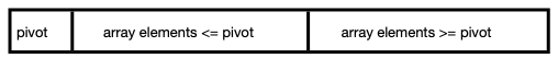
Rearrange elements within an array, so that elements smaller than
the pivot are in the first part of the array, and larger elements at
the end. Elements equal to the pivot can be anywhere. The resulting
array has the form shown in the following schematic:
-
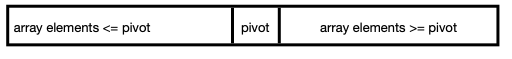
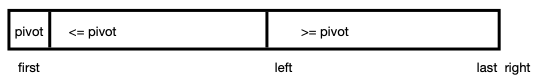
Swap the pivot with the last of the smaller elements. (After
this step, all elements before the pivot have <= values and all
elements after have >= values. Thus, the pivot will be in its correct
location if/when the overall array is sorted.) This final result of
the partition procedure has the form shown in the next schematic:
Since step 1 involves only a decision to identify the pivot (i.e.,
as the first array element) and step 3 involves only a swap, the
overall efficiency of this algorithm depends on rearranging array
elements quickly. In most [all?] implementations, the idea is to
proceed with a simple loop that examines array elements only once.
In all cases, the loop must seek to
- move large elements to the left, and
- move small elements to the right.
Overall, the loop will need to examine successive array elements and
determine whether they belong to the left (small) or right (large) grouping.
Thus, as processing proceeds, the procedure will have to keep track
of three groups: the collection of small elements, the large
elements, and the unprocessed elements (that have not been yet been
placed in a group).
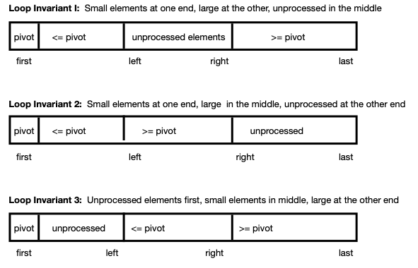
Several variations for implementing the partition procedure differ
in the locations of the small, large, and unprocessed elements, as
shown in the following schematic diagram.
Although it is common to use the leftmost array element as the
pivot, exactly the same approach could be followed using the
rightmost array element, and discussions on some Web sites follow
this alternative viewpoint, Effectively, the potential invariants
of either approach are the mirror image of each other, and both
perspectives can use parallel logic.
Loop Invariant 1: Small Elements first, Then Large, then
Unprocessed
With Loop Invariant 1, the idea is to place small elements at the
start of the array, just after a[first] and to place large elements
at the end of the array. Elements that have yet to be examined are
in the middle. As processing proceeds, the middle section gets
successively smaller, until all elements have been put into the
correct section.
As indicated in the following schematic,
variables first and last identify the
indices of the array segment being processed, and
variables left and right mark the edges of
the known small and large collections.
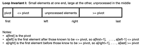
Note:
-
left represents the element just after the known
collection of small items, and and right
represents the element just before the known large elements.
Thus, a[left-1] <= pivot (unless no small
items have yet be identified), and a[left] is
either unprocessed or >= pivot (if no unprocessed elements
remain). Similar statements apply to a[right]
and a[right+1].
Code implementing Loop Invariant 1 largely follows one of two
approaches.
- Examine unprocessed elements down from the right and up from
left—swapping only when a misplaced large and small element is
identified.
- Work through unprocessed elements from one end only (e.g., work
down from the right).
Implementation A: Examine Elements from both ends of the Unprocessed Segment
This traditional approach works from both ends of the array segment
toward the middle, comparing data elements to the first element and
rearranging the array as necessary. This idea is encapsulated in the
following diagram, which is repeated from above.
To implement this approach, we move left and right toward the middle
— maintaining the loop invariant with each step.. The details
follow:
-
Compare a[first] to a[last], a[last-1], etc. until an element a[right] is
found where a[right] < a[first].
-
Compare a[first] to a[first+1], a[first+2], etc. until an element a[left]
is found where a[left] > a[first].
-
Swap a[left] and a[right].
At this point,
-
a[first] < a[right], a[right+1], ..., a[last], and
-
a[first] > a[first+1], ..., a[left]
-
Continue steps A and B, comparing the original first element against
the end of the arrays, until all elements of the array have been checked.
-
Swap a[first] with a[right], to put it in its correct location.
These steps are illustrated in the following diagram:
The following code implements this basic step:
int left=first+1;
int right=last;
int temp;

while (right >= left) {
    // search left to find small array item
    while ((right >= left) && (a[first] <= a[right]))
        right--;
    // search right to find large array item
    while ((right >= left) && (a[first] >= a[left]))
        left++;
    // swap large left item and small right item, if needed
    if (right > left) {
        temp = a[left];       // swap a[left] and a[right]
        a[left] = a[right];
        a[right] = temp;
    }
}
// put a[first] in its place
temp = a[first];              // swap the pivot, a[first], and a[right]
a[first] = a[right];
a[right] = temp;
Efficiency Notes:
-
Several published sources of this algorithm use a
separate swap procedure to
interchange a[left] and a[right] and to
interchange a[first] and a[right].
Although this coding is correct and may look clean, the actual
effect adds a separate procedure call for every swap. In practice,
the time for each call accumulates and can slow the runtime for the
algorithm noticeably. Writing out the lines for the swap, rather
than calling a procedure, can improve performance.
-
This implementation swaps elements only when both a small and
large element are known to be out of place. No additional
data movements are utilized, enhancing the efficiency of this
approach.
Implementation B: Examine elements from one end of the Unprocessed
Segment Only
In this approach, seen in a number of YouTube videos, processing
proceeds downward from the top end of the array toward the pivot.
The details follow:
-
Compare a[right] with the pivot.
- If a[right] >= pivot, decrease right, and continue.
- If a[right] < pivot, swap a[right] and a[left], increase
left, and continue.
Altogether, the collection of large elements is expanded whenever a
large element is found, and the collection of smal elements is
expanded whenever a small element is found.
Although the swap process can be written out within the partition
procedure, this approach sometimes (often?) is written with a call
to a swap function. This produces the following code:
  int pivot = a[first];
  int left;
  int right = last;

  for (left = first+1; left <= right;) {
    if (a[left] < pivot) {
      left++;
    }
    else {
      swap (&a[left], &a[right]);
      right--;
    }
  }

  swap (&a[first], &a[right]);
Efficiency Notes:
-
Since processing examines only one end of the unprocessed array
elements, swaps occur every time a small element is identified at
the far unprocessed end. However, since the other end of the
unprocessed segment is not examined, the swap may exchange one
small element for another. The array segment for small elements
is expanded, but the next iteration may require another swap.
Altogether, many unnecessary swaps may be made, decreasing the
efficiency of this approach.
-
As noted above, use of a swap function may yield a
simple-looking procedure, but can add considerable overhead with many
potential procedure calls. A typical implementation follows:
  // swap procedure
void swap (int * a, int * b) {
  int temp = * a;
  * a = * b;
  *b = temp;
}
Loop Invariant 2 with Small Elements on Left; Large Elements
Next
In this approach, the idea is to maintain small elements and then large
elements toward the start of the array. The right of the array contains
elements that are yet to be examined. As processing proceeds, the right
section shrinks until all items are in their appropriate section.
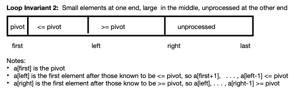
During processing, we compare successive items in the array to a[first].
- left marks the array index after the checked array that are less than
or equal to a[first]
- right marks the index of the block of array of items that have not
been examined yet.
Examining this picture in more detail, at the start, there are no examined
items, so there are no items that we know are <= a[first] and also no
items that we know are > a[first], as shown in the following diagram:
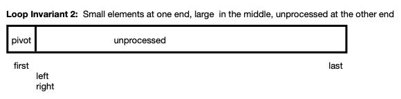
This picture suggests the following initialization:
   left = first + 1;
   right = first + 1;
Once processing has begun, we examine the unprocessed element a[right].
-
If this element is larger than a[first], the loop invariant (and figure)
can be adjusted by expanding the > a[first] section: right++
-
If this element is less than or equal to a[first], then we need to move it
to the collection of small items. A simple way to do that is to swap
a[left] and a[right] and increment both left and right.
Processing continues until all items are processed, as shown in the
following diagram:
Based on this outline, the entire code for placing a[first] in its correct
position is:
   // progress through array,
   //     moving small elements to a[first+1] .. a[left-1]
   //     and moving large elements to a[left] .. a[right-1]
   while (right <= last)
     {
       if (a[first] < a[right])
          right++;
       else {
          // swap a[left] and a[right]
          temp = a[right];
          a[right] = a[left];
          a[left] = temp;
          left++;
          right++;
       }
     }
    // put a[first] in its place
    temp = a[first];
    a[first] = a[left-1];
    a[left-1] = temp;
Efficiency Notes:
-
As small elements are found, they are added to expand the
collection on the left, by swapping them with an element already
found to be large. Thus, swapping is required for every small
element; large items therefore may move several times as new small
ones are found.
-
As discussed previously, replacing the three lines for
swapping elements by a single call to a swap
procedure can make the code look simpler, but such an approach
adds the overhead of more procedure calls.
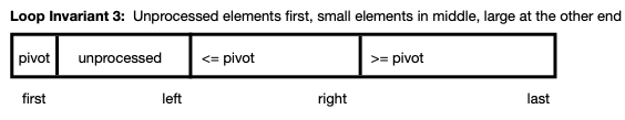
Loop Invariant 3 with Unprocessed Elements coming before Small and
Large elements
In this approach, the segment of unprocessed elements is located
immediately after the pivot, with the segments for small and then
large elements following.
Effectively, processing for this invariant can be viewed as the
mirror image of that for Loop Invariant 2. In this case, processing
begins at the right end of the array (with
element a[last]) and proceeds toward the beginning of
the array. In this processing,
- when small elements are found, the collection of small elements
can be expanded.
- when large elements are found, they must be swapped with small
ones at the far end of the small collection (at index right), as a means to expand
the large collection
With the similarities between the processing for Loop Invariants 2
and 3, further details and the code for Loop Invariant 3 are left to
the reader.
Implementing Quicksort
Regardless of the loop invariant used for a partition function, a
pivot is identified and other array elements are moved as needed, so
that the pivot can be placed after all amaller (or equal) array
elements and after all larger (or equal) elements. This positioning
of elements is shown in the following schematic, repeated from
earlier in this reading:
As part of processing, the new location of the pivot is known and
thus could be returned by a partition function.
Based on this partition function, sorting can proceed by applying
the partition procedure to the entire array and then recursively to
the first and last parts of the array. The base case of the
recursion arises if there are no further elements in an array
segment to sort.
This gives rise the the following code, called a quicksort.
int partition (int a[ ], int size, int left, int right) {
  int pivot = a[left];
  int l_spot = left+1;
  int r_spot = right;
  int temp;

  while (l_spot <= r_spot) {
    while( (l_spot <= r_spot) && (a[r_spot] >= pivot))
      r_spot--;
    while ((l_spot <= r_spot) && (a[l_spot] <= pivot))
      l_spot++;

    // if misplaced small and large values found, swap them
    if (l_spot < r_spot) {
      temp = a[l_spot];
      a[l_spot] = a[r_spot];
      a[r_spot] = temp;
      l_spot++;
      r_spot--;
      }
  }

  // swap a[left] with biggest small value
  temp = a[left];
  a[left] = a[r_spot];
  a[r_spot] = temp;

  return r_spot;
}
void quicksorthelper (int a [ ], int size, int left, int right) {
  if (left > right)
    return;
  int mid = partition (a, size, left, right);
  quicksorthelper (a, size, left, mid-1);
  quicksorthelper (a, size, mid+1, right);
}

void quicksort (int a [ ], int n) {
  quicksorthelper (a, n, 0, n-1);
}
As shown in this implementation, the full code for the quicksort
involves three procedures:
-
The quicksort procedure supports a user's
view of sorting; the user wants to sort an array of a given length
and does not care about the implementation details.
-
quicksortHelper: A programmer needs to apply
the partition function recursively to various parts of
the array. Thus, from a programmer's
perspective, partition must know the indices of the
start and end of the array segment to be processed. To accomplish
this, the programmer needs a helper function,
called quicksortHelper, with the needed
parameters.
-
partition: Behind the scenes moving elements within
the array is handled by partition, as discussed
earlier.
Analysis and Timing
The quicksort is called a divide-and-conquer algorithm, because the
first step normally divides the array into two pieces and the approach is
applied recursively to each piece.
Suppose this code is applied an array containing n randomly ordered data.
For the most part, we might expect that the quicksort's divide-and-conquer
strategy will divide the array into two pieces, each of size n/2, after the
first main step. Applying the algorithm to each half, in turn, will divide
the array further -- roughly 4 pieces, each of size n/4. Continuing a
third time, we would expect to get about 8 pieces, each of size n/8.
Applying this process i times, would would expect to get about
2i pieces, each of size n/2i.
This process continues until each array piece just has 1 element in it,
so 1 = n/2i or 2i = n or i = log2 n.
Thus, the total number of main steps for this algorithms should be about
log2 n. For each main step, we must examine the various array
elements to move the relevant first items of each array segment into their
correct places, and this requires us to examine roughly n items.
Altogether, for random data, this suggests that the quicksort requires
about log2 n main steps with n operations per main step.
Combining these results, quicksort on random data has O(n log2
n).
An Improved Quicksort
A basic quicksort algorithm typically chooses the first or last element in
an array segment as the point of reference for subsequent
comparisons. (This array element is often called the pivot.)
This choice works well when the array contains random data, and the work
for this algorithm has O(n log n) with random data.
However, when the data in the array initially are in ascending order or
descending order, the analysis of efficiency breaks down, and the quicksort
has O(n2). (The analysis is much the same as insertion sort for
data in descending order.)
To resolve this difficulty, it is common to select an element in the array
segment at random to be the pivot. The first part of the quicksort
algorithm then follows the following outline:
private static void quicksortKernet (int[] a, int first, int last)
{
   pick an array element a[first], ..., a[last] at random
   swap the selected array element with a[first]

   continue with the quicksort algorithm as described earlier
   ...
}
With this adjustment, quicksort typically performs equally well (O(n log
n)) for all types of data.
A Hybrid Quicksort
For the most part, the divide-and-conquer approach of quicksort can
be very efficient. Large segments of an array are repeatedly
divided in half. This allows the algorithm to utilize roughly
O(log2 n) levels of processing, and the
quicksort (usually) runs in time O(n log2n). However,
near the bottom of the recursion, calls to partition
can be made to sort array segments with only a few data elements.
In such circumstances, the overhead of calling a function may
dominate any gain from array processing.
To address such matters, a hybrid approach can be considered. The
idea is:
- in the recursive step
- if the number of elements in an array segment is small
- use an insertion sort
- else use partition and the usual quicksort.
Since large array segments are divided in half during processing,
this approach retains the speed of a quicksort, but avoids numerous
function calls on small array segments. In practice, some
experimentation may be needed to determine when an insertion sort
should be called.
